Reduction
Manual Reduction
Terminal command reduce_REF_M is available on the pixi environments mr_reduction_qa and mr_reduction.
Running this command starts a simple web application to configure reduction of a single experiment.
Developers or power users running their own pixi environment by cloning the repository,
and installing by running pixi install
can invoke the webapp by running script src/mr_autoreduce/reduce_REF_M_run.sh
> reduce_REF_M
**********************************************
* POINT YOUR BROWSER TO http://127.0.0.1:5000/
**********************************************
[2024-07-09 11:20:06 -0400] [278702] [INFO] Starting gunicorn 21.2.0
[2024-07-09 11:20:06 -0400] [278702] [INFO] Listening at: http://0.0.0.0:5000 (278702)
[2024-07-09 11:20:06 -0400] [278702] [INFO] Using worker: sync
[2024-07-09 11:20:06 -0400] [278707] [INFO] Booting worker with pid: 278707
As the printout suggests, open a tab in your browser and enter address http://127.0.0.1:5000/.
This webapp allows one to reduce a single run by entering the Nexus events file, entering the directory
storing the reduced files, and selecting reduction options.
Hovering over the bold-face text items will show explanatory tooltips.
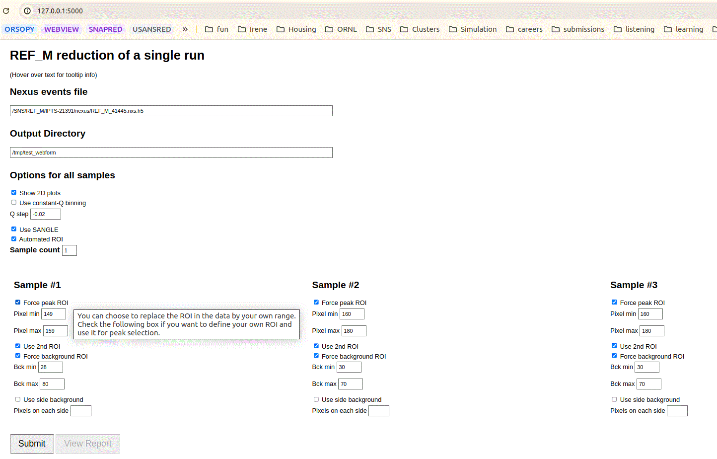
Configuration for manual reduction.
Click on the Submit button to start reduction. The reduction typically takes one to two minutes during which time both Submit and View Report buttons became disabled. After reduction is finished, click on View Report for a summary of the results.
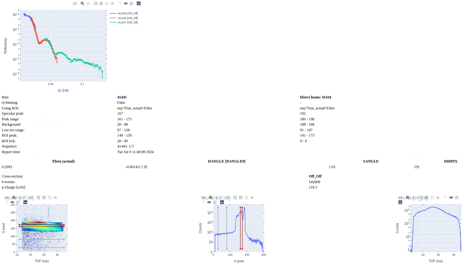
Report for the manual reduction.
The report shown is HTML file /tmp/test_webform/REF_M_REF_M_41445.html, where /tmp/test_webform/ is the
output directory we selected.
Notice how the report shows the superposition of reflectivity curves for runs 41445, 41446, and 41447. This
will happen if reduced files for runs 41446 and 41447 are found either in the output directory /tmp/test_webform
or the canonical output directory for autoreduction of runs corresponding to run 41445 which in this
case is /SNS/REF_M/IPTS-21391/shared/autoreduce/. Runs 41445, 41446, and 41447 correspond to experiments
taken on the same peak but with a different incidence angle.
Reduction of a Sample with Two Peaks
The webapp supports reduction of up to three peaks for the scenarios when the run contains more than one peak. This typically arise when the sample has layers with slightly different orientations with respect to the incoming beam. Thus, the layers will reflect neutrons at slightly different angles. This results in distinct intensity regions (peaks) in the detector panel.
The picture below shows two runs (42536 and 39012) each one reflecting two distinct intensity regions.
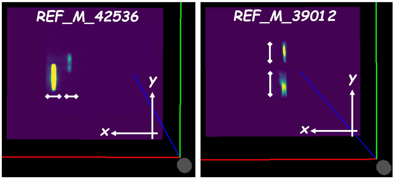
For run 42536, identifying two distinct ranges along the X-axis suffices to differentiate the two peaks. For run 39012, two distinct ranges along the Y-axis suffice to differentiate the two peaks.
We’ll reduce the run series 43884 and 43885. These runs contain two peaks as shown in the figure below for run 43885.
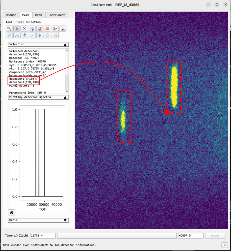
We should start with the first run of the series, in this case run 43884, by invoking the webapp from the terminal. Even though the two peaks are well resolved along the X-axis, we’ll also define a range along the Y-axis, also termed the low-resolution axis because the peak is spread out over many pixels along this direction.
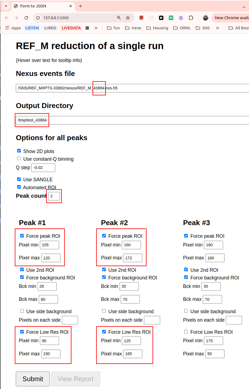
A few things to notice in the above figure:
We pass the path to the events file for run 43884.
We set up the output directory. If the directory doesn’t exist, do create it before submitting the form.
We specified the peak count to two peaks.
For Peak #1, we specified the range along the X-axis (“Force peak ROI”) as well as the Y-axis (“Force Low Res ROI”).
We do likewise for Peak #2.
We start the reduction by pressing the Submit button. After the reduction is finished, we can view the report by pressing the View Report button:
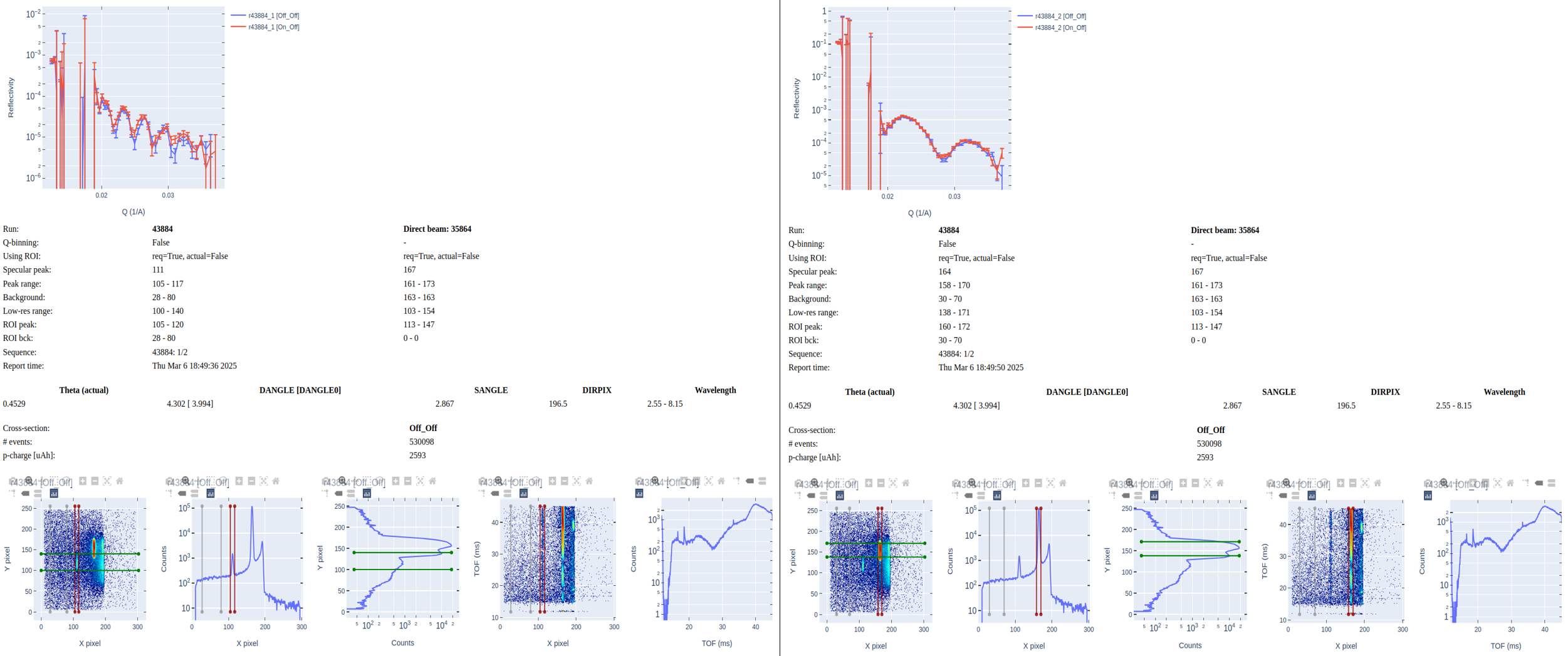
The report shows the reflectivity of the two cross-sections (“Off_Off” and “On_Off”) for Peak #1 (“43884_1”) and Peak #2 (“43884_2”).
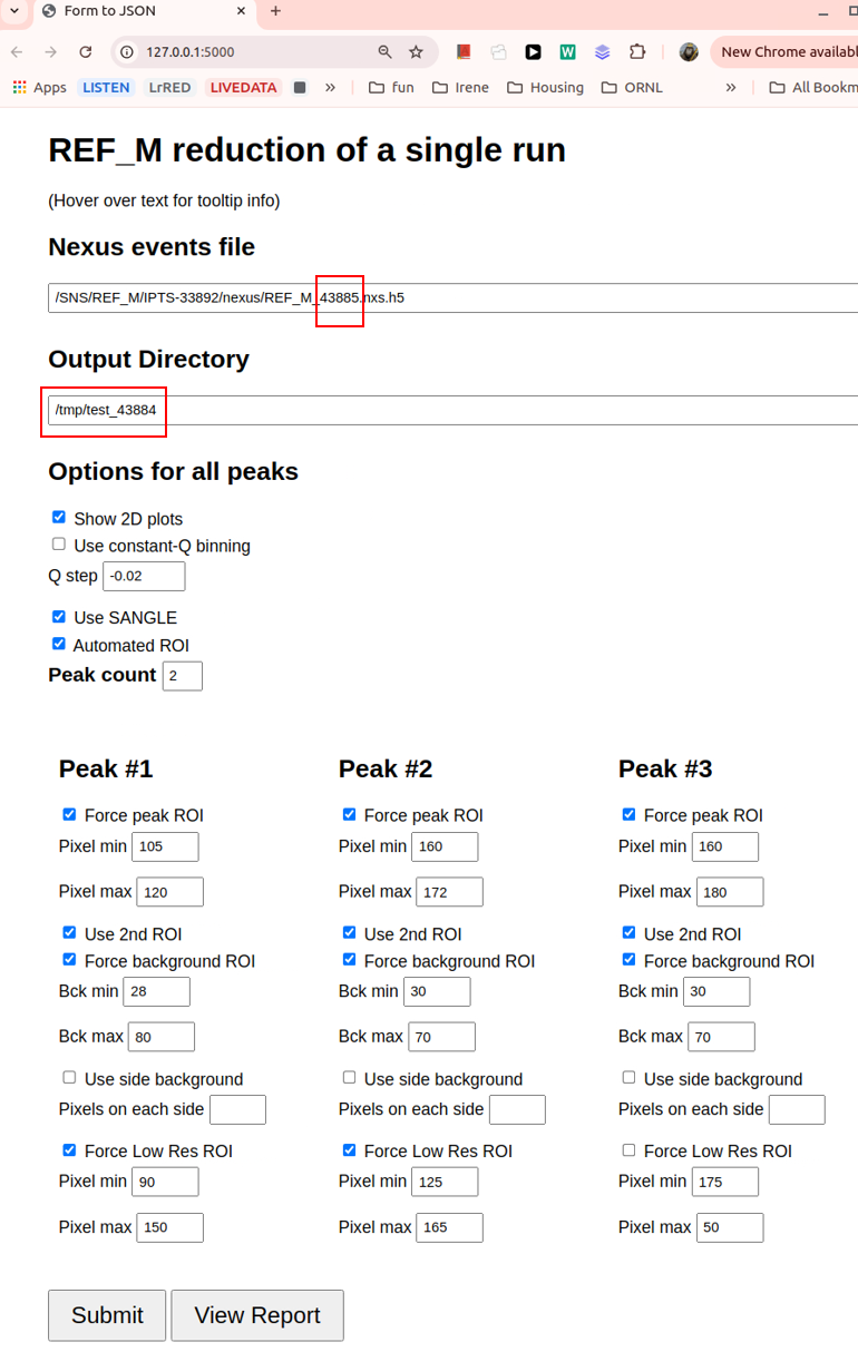
We continue by reducing the second run in the series (43885). The only change we make in the form is to pass the path to the events file for run 43885. Beforehand we made sure that the ranges for “Force peak ROI” and “Force Low Res ROI” that we used when reducing 43884 also encompass the peaks observed in run 43885. Notice that we will output the reducted data to the same directory as for run 43884. This way we’ll have all the necessary output data to stitch together the reflectivity curves of the two runs.
As before, we view the report by pressing the View Report button:
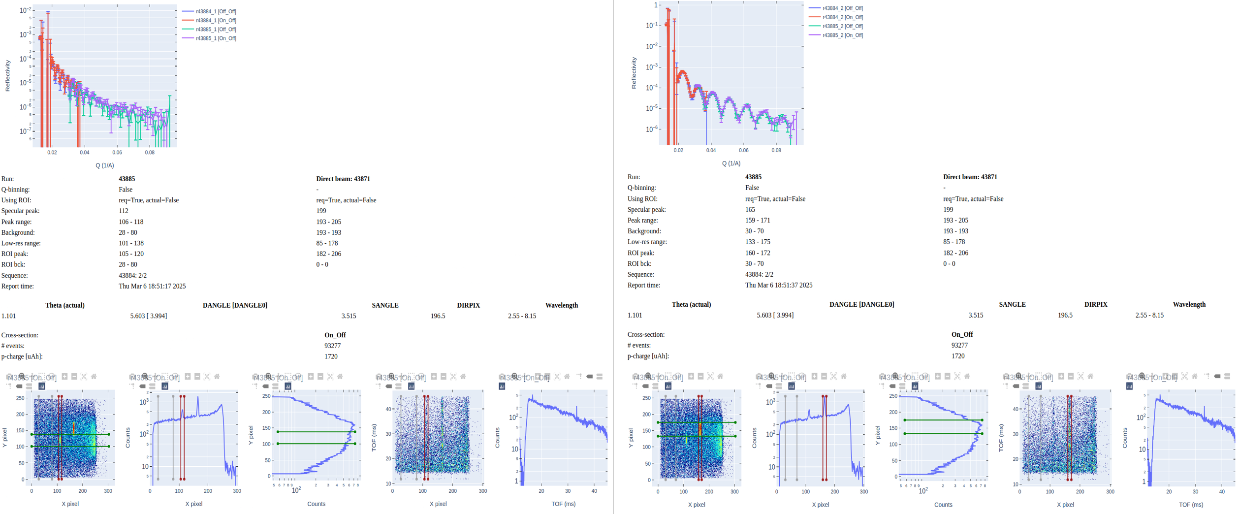
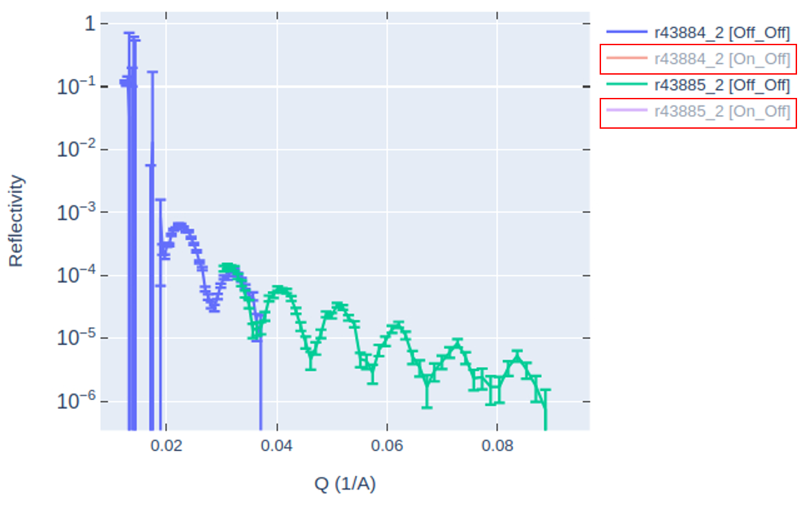
We notice in the report that reflectivity curves for the two runs are shown, stitched together. There are four curves in each plot so it can be difficult to discern the stitching for a given cross-section. You can hide one curve by clicking on the legend. In the figure below, on the legend, I clicked on “r43884_2 [On_Off]” and “r43885_2 [On_Off]” to hide them, leaving a clearer view of the stitching for the “Off_Off” cross-section.
In the output directory,
the files containing the reflectivity curves in ASCII format are REF_M_*_autoreduce.dat
for individual runs and REF_M_*_combined.dat for stitched runs.
Automated Reduction
The set of reduction options available in the manual reduction is also available in
https://monitor.sns.gov/reduction/ref_m/. Updating these options ensure that auto-reduction
of future experiment will employ the new options.
Auto-reduced files are saved under directory /SNS/REF_M/IPTS-XYZ/shared/autoreduce/, where XYZ corresponds
to the IPTS number associated to whatever run number is to be auto-reduced.
Output Files
After successful completion of the autoreduction, the following files are generated in the output directory. Belows is a list for run peak 42535_1. The particular cross-sections will depend on the instrument settings, which for run peak turn out to be “Off_Off” and “On_Off”.
REF_M_42351.html: HTML report summarizing the results of the auto-reduction.
REF_M_42535_1_Off_Off_autoreduce.dat: reflectivity curve for the “Off_Off” cross-section.
REF_M_42535_1_Off_Off_autoreduce.nxs.h5: reflectivity curve for the “Off_Off” cross-section (Nexus format) with all sample-logs of the original Nexus events file.
REF_M_42535_1_On_Off_autoreduce.dat: reflectivity curve for the “On_Off” cross-section (ASCII format).
REF_M_42535_1_On_Off_autoreduce.nxs.h5: reflectivity curve for the “On_Off” cross-section (Nexus format) with all sample-logs of the original Nexus events file.
REF_M_42535_1.ort: reflectivity curves for all cross-sections (ORSO ASCII format).
REF_M_42535_1_partial.py: python script to autoreduce run peak 42535_1.
REF_M_42535_1_Off_Off_combined.dat: combined reflectivities for the “Off_Off” cross-section for all runs in the same run-sequence as 42535. Run 42535 is the first run in the sequence, hence is endowed with the combined file.
REF_M_42535_1_On_Off_combined.dat: combined reflectivities for the “On_Off” cross-section for all runs in the same run-sequence as 42535. Run 42535 is the first run in the sequence, hence is endowed with the combined file.
REF_M_42535_1_combined.ort: combined reflectivities for all cross-sections for all runs in the same run-sequence as 42535 (ORSO ASCII format).
REF_M_42535_1_combined.py: paste scripts
REF_M_*_partial.pyfor all runs in the same run-sequence as 42535.REF_M_42535_1_tunable_combined.py: same as
REF_M_42535_1_combined.py, but the reduction workflow of each run is grouped into two functions, one splitting the events according to the cross-section and the other to calculate the reflectivity curve for each cross-section.REF_M_42535_1.json: a small “database” file storing the path to the nexus file as well as the names of the cross-section reflectivity files
REF_M_42535_1_*_autoreduce.dat.
Live Reduction
Reduction of data as is being taken during the experiment is termed as “live reduction”. A live reduction service has been installed in a dedicated virtual machine, bl4a-livereduce.sns.gov, for live reduction of BL4A (a.k.a REF_M) data. The service taps into the ADARA data stream and attaches a Mantid live listener to the data stream. The main Mantid algorithm for live reduction is LoadLiveData. This algorithm creates child algorithm RunPythonScript and runs it in a separate python interpreter process as
RunPythonScript(InputWorkspace=input,
                Filename="/SNS/REF_M/shared/livereduce/reduce_REF_M_live_post_proc.py")
where input is the EventWorkspace
containing the events accumulated up to the time when script reduce_REF_M_live_post_proc.py is run.
Package mr_reduction.mr_livereduce contains script
reduce_REF_M_live_post_proc.py
which specifies all the steps for successful reduction of the accumulated events workspace input.
Live-reduction is very similar to auto-reduction, thus script
reduce_REF_M_live_post_proc.py
reuses much of the functionality encoded in the template auto-reduction script
mr_reduction.mr_autoreduce.reduce_REF_M.py.template.
When the live-reduction script is deployed as /SNS/REF_M/shared/livereduce/reduce_REF_M_live_post_proc.py
and invoked as above, the script imports the deployed auto-reduction script
/SNS/REF_M/shared/autoreduce/reduce_REF_M.py as if it were a python module.
This way the functions defined in the auto-reduction script can be reused in the live-reduction script.
The output of the live-reduction script is virtually identical to that of the auto-reduction script, namely a series of reduced files and an HTML report that is saved to the output directory and uploaded to the live data server and available in the monitor web page. The only difference is that the live-reduction report contains two graphs missing in the autor-reduction report. The graphs inform on the spin flipping ratio and the normalize spin differences.
Tips for Live Reduction Scripts
To avoid having auto-reduction and live-reduction scripts stepping on each other’s toes,
it is recommended to check for the existence of the Nexus data files before attempting to reduce them.
Live reduction should only reduce active runs, i.e. runs that are still being taken, while auto-reduction
should only reduce completed runs.
This can be done using the os.path.exists() function in python, for example:
import os

ipts = SampleLogs(input_workspace)["experiment_identifier"]  # e.g. 'IPTS-31954'
nexus_filepath = f"/SNS/REF_M/{ipts}/nexus/{run_number}.nxs.h5"

 # if the run NeXus file exists, live reduction should not proceed
 if os.path.exists(nexus_filepath):
     api.logger.error(f"Post-Processing: NeXus file exists: {nexus_filepath}")
     return

# proceed with live reduction
This way the live-reduction script can safely skip any runs that have already been processed by the auto-reduction script.